Managerial Economics (ECN7302) - Megan Way, mway@babson.edu, x5892
Session 1: Oct 25th, 2011
Economics: Study allocation of scarce resources.
Economic systems are set up to allocate scarce resources
Individuals are trying to maximize - utility
Firms are trying to maximize - profits
Govts are trying to maximize - welfare
Consumers:
Rational choice, we assume rational.
Traditional economics assume that people are rational., (There is new concept of behavioral economics in which people somewhat do not behave rationally)
Utility:
satisfaction, happiness, value to consumer
Marginal utility:- utility from teh next unit of teh good
Diminishing MU:- more consumed in a time period lowers the utility of teh next unit.
How do we measure utility: by either bringing in units like "Util" OR we rank it against something else
Maximizing utility subject to:
Session 2: Oct 27, 2011
Discussion on the assignment.
Session 3; Nov 1, 2011
Assignment
Session 1: Oct 25th, 2011
Economics: Study allocation of scarce resources.
Economic systems are set up to allocate scarce resources
- Centralized common control (USSR, North Korea)
- Mixed market
- We let the market function
- give regulation, provisioning of some goods etc.
- Free market
questions:
- What is produced?
- How is it produced?
- Who is it produced for?
Individuals are trying to maximize - utility
Firms are trying to maximize - profits
Govts are trying to maximize - welfare
Consumers:
Rational choice, we assume rational.
Traditional economics assume that people are rational., (There is new concept of behavioral economics in which people somewhat do not behave rationally)
Utility:
satisfaction, happiness, value to consumer
Marginal utility:- utility from teh next unit of teh good
Diminishing MU:- more consumed in a time period lowers the utility of teh next unit.
How do we measure utility: by either bringing in units like "Util" OR we rank it against something else
Maximizing utility subject to:
- preferences -
- assume that they are complete (you will never say i dont know)
- assume that the preferences are transitive
- assume that "more is better"
- assume (preferences are stable over time)
- income
- prices of all goods
Then we move to the discussion of indifference curves for the utility. See page 5 of lecture notes.
Bring in the budget constraint now.
The budget constraint is a straight line with decreasing slope when drawn with Price of Q1 on y and price of Q2 on y.
Draw an indifference curve on top of the budget constraint line. Move to the point where indifference curve is tangent to the budget constraint line.
At equilibrium (when you have maximized utility) your MRS (marginal rate of substitution) will be = -Px/Py [only at equilibrium]
otherwise marginal rate of substitution MRS = delta Qy/ delta Qx
What can you as a marketing person to influence the equilibrium point.
either change the price to change the slope of the budget contraint line. OR do advertisement to change the utility curve.
Session 2: Oct 27, 2011
Discussion on the assignment.
Session 3; Nov 1, 2011
Assignment
1. Mr. Smith has the following
demand equation for a certain product:
Q
= 30 - 2P.
a) At a price of $7, what is
the point elasticity?
Ans: P=7 => Q = 30 - 14 = 16
point elasticity = dQ/dP * P/Q
dQ/dP = -2
P/Q (at P=7) = 7/16
PED = -7/8 = -0.87
Interpretation: if i raise the price by 1% the quantity demanded will go down by 0.87%
b) Between prices of $5 and $6, what is the arc elasticity?
Ans: at P=5; Q=20 and at P=6; Q=18
E = delta Q / delta P * (P1 +P2) / (Q1+Q2) ; (20-18)/(-1)*(6+5)/(18+20) = -11/19 = -0.579
Interpretation: if i raise the price by 1% the quantity demanded will go down by 0.579%
c) If the market is made up of 100 individuals with demand curves identical to Mr. Smith’s, what are the point and arc elasticities for the conditions specified in parts a and b?
no change
Interpretation: because the elasticities are calculated in terms of %ages, we have eliminated the number of products sold from our equation that way.


Session 4: Nov 3, 2011
Production and cost theory
Production function, Q = f|(K,L)
K refers to fixed capital, its not just the $
short run vs the long run
short run = time period in which at least one input is fixed
long run = all inputs vary
Q = Total product (TP)
APL = TP/L = Q/L
MPL = delta TP/ delta L = delta Q / delta L
Diminishing Marginal Returns: As you add variable input to a fixed input you hit point where variable input is less productive
W/APL = Avg cost
e.g. W/APL Germany < W/APL Greece (even though the wages are higher in Germany)
Cost Terminology
Accounting costs: explicit
Economic costs: explicit + implicit
explicit: monetary outlays
implicit: foregone earnings (opportunity costs)
implicit: what you could earn with the next best use of your resources
sunk cost:
anything that increases productivity decreases cost
SO the cost functions and the productions are a mirror image of each other.
Total Cost Tc = FC + VC
ATC = TC/Q ; AFC FC/Q ; AVC = VC/Q ; MC = delta TC / delta Q
Profits = (P-ATC)*Q
Breakeven point = where MC intersects the ATC
Shutdown rule P<AVCmin
shutdown point is the minimum AVC
Session 5: Nov 8, 2011
Session 6: Nov 10,2011
Salem Telephone company
Variable costs:
Power - $4.7/hr
hourly staff - $ 24.00
AVC = 28.7
(P-AVC) contribution
800-28.7 = 771.30 (hourly cont commercial)
400-28.7 = 371.30 (hourly cont intra-company)
Total fixed cost = 212,000 (add all except the variable costs)
Total fixed cost not covered by intra-company sales
= 212000 - 205(400 - 28.7)
= 136,900
break-even quantity, Q = 136,900/(800-28.7) = 177 hours
------------------------------------
Lets calculate elasticities for Salem
Arc elasticity
P1 = 800, P2 = 1000
Q1 = 138, Q2 = 97
Arc elasticity = -1.57021 (in the elastic range)
P2 = 600
Q2 = 179
Arc elasticity = -0.9 (in the inelastic range)
For
TR =
Session 7: Nov 15, 2011
Degree of Operating leverage
DOL = % change in profit / % change in Q
assuming no pricing power and constant AVC
=> profit = (P-AVC) * delta Q / (P-AVC-AFC) * Q
= (P-AVC)
if operating leverage is higher .. you have higher profit potential after the breakeven point but at the same time below the breakeven point the loss potential is also higher.
Externalities
Negative externality - cost is borne by society.
Session 12: Dec 1, 2011
Palm has decided to pursue a price discrimination
policy that supports short-run profit maximization (skimming) for each of the two
new markets. Use this information to
calculate the profit-maximizing quantities and prices for Europe and Asia. (In calculating coefficients, please use five
decimal places).
VC = AVC*Q
VC = 220Q
MC = dVC/dQ = 220
For Europe
Pe = 900 - 0.00225Q
MR = 900 - 0.0045Q
at profit maximization MR = MC
900 - 0.0045Q = 220
Qe = 151,109
Pe = 560
Contribution:
per unit:560 - 220 = 340
total = 51,377,060
Asia
Pa = 725 - 0.0009Q
MR = 725 - 0.0018Q
at MR = MC
725 - 0.0018Q = 220
Qa = 275,354
Pa = 474
Contribution/unit: 474 - 220 = 254
total: 69,939,916
Total Asia and Europe = 120,643,627
--------------
part b)
combined demand equation:
Q = 1190622 - 1535P
P = 776 - 0.0006Q
MR = 776 - 0.0013Q
MR = MC
776 - 0.0013Q = 220
Q = 427,438
P = 497.84
Contribution: 497.84 - 220 = 277.84
total cont = 118,759,373.92
-----------------------
Assume that the arc price elasticity (from part a.) is
the best available estimate of the point price elasticity of demand. If marginal cost is $135 per unit for labor
and material, calculate TLC’s optimal markup on price and its optimal
price. Comment on TLC’s current prices.
P1 = 250
P2 = 200
Q1 = 3,250
Q2 = 5,750
elasticity = [delta Q / delta P ]*[(P1+P2)/(Q1+Q2)]
elasticity = -2.5
Assume that the arc price elasticity (from part a.) is the best available estimate of the point price elasticity of demand. If marginal cost is $135 per unit for labor and material, calculate TLC’s optimal markup on price and its optimal price. Comment on TLC’s current prices.
M (Optimal markup) =[ -1/(1 - |elasticity|)]*MC
1 + M = E/(1+E)
TLC arc E = -2.5
1+M = -2.5/(1-2.5) = 1.667
M = 0.667
M = 66.7%
MC = 135
M = 66.7%
Session 14: Dec 6, 2011
Case; P&G - Wal-mart partnership
Diaper market:
Characteristics - elasticity
Luxury vs necessity - inelastic
number of substitutes - cloth - inelastic
% of budget - relatively high - elastic
Time frame
Market structure
- Differentiated
- # of firms - few (3-4)
- Barriers to Entry - high, R&D, high FC, economies of scale, distribution, brand
- Pricing power - decide their own price
- Interdependence
Oligopoly
Apply game theory on the case
Kimberly Clarke and P&G have options of either go premium or promotional pricing
P&G, KC
dQ/dP = -2
P/Q (at P=7) = 7/16
PED = -7/8 = -0.87
Interpretation: if i raise the price by 1% the quantity demanded will go down by 0.87%
b) Between prices of $5 and $6, what is the arc elasticity?
Ans: at P=5; Q=20 and at P=6; Q=18
E = delta Q / delta P * (P1 +P2) / (Q1+Q2) ; (20-18)/(-1)*(6+5)/(18+20) = -11/19 = -0.579
Interpretation: if i raise the price by 1% the quantity demanded will go down by 0.579%
c) If the market is made up of 100 individuals with demand curves identical to Mr. Smith’s, what are the point and arc elasticities for the conditions specified in parts a and b?
no change
Interpretation: because the elasticities are calculated in terms of %ages, we have eliminated the number of products sold from our equation that way.
2. Deck
& Blacker (DB) makes small kitchen appliances. DB hired a consulting economist to estimate
the demand for toaster ovens. The
consultant used data gathered from DB’s sample market survey.
Qx =
40 - 1.1Px +
0.1Pc + 0.32I
+ 1.5Ax
(2.06) (.06)
(.003) (4.31) (.5)
Qx
is the quantity demanded in thousands; Px
is the price in dollars; Pc
is the price of leading competitor; I is the mean household income, measured in
thousands; Ax is the company
advertising expenditure (measured in thousands of dollars). (Note: The figures in parenthesis are
standard errors of the coefficients. The
regression analysis also provided the coefficient of determination, which is
0.75. This information can be omitted in
answering the questions below.)
The current
values of the independent variables are:
Px = 55; Pc = 50; Ax = 20; and I =
31. Please answer the following
questions:
a) Current level of sales, Qx , is: 40 - 1.1(55) + 0.1(50) + 0.32(31) + 1.5(20) = 24.42
b) point elasticity = -1.1* 55/24.42 = -2.4 (if i lower my price by 1% quantity demanded will go up by 2.4% so yes we should consider lowering the price for higher revenues.
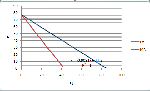
c) What is the total revenue maximizing price for
Deck & Blacker toaster ovens? Graph
the demand and marginal revenue curves.
Plot the revenue maximizing price and output.
Ans: Qx = f(Px,Pc,I,A)
Qx= f(Px) (keeping all teh rest of the variables constant)
Qx= 40 - 1.1(Px) + 0.1(50) +32(31) =1.5(20)
Qx = 84.92 - 1.1Px
Qmax = 84.92
=> P = 77.2 - 0.91Qx
Total Revenue, TR = P * Q
TR = (77.2 - 0.91Qx)*Qx
TR = 77.2Qx - 0.91Qx^2
dTR/dQx = 77.2 - 2(0.91)Qx
dTR/dQx = 77.2 - 1.82Qx
Marginal Revenue = dTR/dQx
Total revenue is maximum at the tangent when MR = 0
So, put dTR/dQx = MR = 0 and solve for Qx
77.2 - 1.82Qx = 0
-> Qx (max) = 48.46

d) How concerned should DB be about price discounts
by its leading competitor? Explain.
Ans: Price demand by competitor
cross Price elasticity % delta Qb / % delta Pc
elasticity(x,c) = dQ/dPc * Pc/Q
= (0.1)*(50/24.42) = 0.2
elasticity (xc) < 0 complements
elasticity (xc) > substitutes
this implies that teh two products are substitutes
So, if the competitor gives the discount WE SHOULD be concerned
e) How concerned should DB be about the prediction
that the country is slipping into a recession?
Ans: We should be looking at teh income elasticity
elasticity(I) = % delta Q / % delta I = dQ/dI * I/Q = 0.32 * (31/24.42) = 0.406
elasticity(I) > 0 - normal good
elasticity(I) < 0 inferior good
elasticity(I) > 1 luxury good ~ superior good
this implies that since this is a normal good, recession will have a negative effect on our sales->revenues
as
f) How
effective do you think advertising is for this company?
Ans: elasticity(A) = %delta Q / % delta A = dQ/dA * A/Q = 1.5 * (20/24.42) = 1.23
say A1 = 20,000 and A2 = 20,200 (1% increase)
-> Q1 = 24,420 and Q2=(1.0123)*Q1 = 24,720
so this means that an increase of $200 of advertising gives us 300 units of additional sales
lets see the effect on revenue
TR = P*Q
delta TR = 55*300 = 16,500
so this implies an extra spending of $300 will give us an additional revenue of $16,500
---------------------------------------------------------------------
Cost calculations:
Lets say we have Marginal Cost, MC or $20
if we have MC=$20
so to maximize profit, we put MR = MC
77.2 - 1.82Qx = 20
=> Qx = 31.43 this teh quantity which will give us teh maximum profit.
we can get teh price for this quantity
P = 77.2 - 0.91*(31.43)
= $ 48.6
Rule: Profit maximization - MC = MR
Consumer surplus:
There are externalities as well. There are spill overs.
See lecture notes on externalities.
Session 4: Nov 3, 2011
Production and cost theory
Production function, Q = f|(K,L)
K refers to fixed capital, its not just the $
short run vs the long run
short run = time period in which at least one input is fixed
long run = all inputs vary
Q = Total product (TP)
APL = TP/L = Q/L
MPL = delta TP/ delta L = delta Q / delta L
Diminishing Marginal Returns: As you add variable input to a fixed input you hit point where variable input is less productive
W/APL = Avg cost
e.g. W/APL Germany < W/APL Greece (even though the wages are higher in Germany)
Cost Terminology
Accounting costs: explicit
Economic costs: explicit + implicit
explicit: monetary outlays
implicit: foregone earnings (opportunity costs)
implicit: what you could earn with the next best use of your resources
sunk cost:
anything that increases productivity decreases cost
SO the cost functions and the productions are a mirror image of each other.
Total Cost Tc = FC + VC
ATC = TC/Q ; AFC FC/Q ; AVC = VC/Q ; MC = delta TC / delta Q
Profits = (P-ATC)*Q
Breakeven point = where MC intersects the ATC
Shutdown rule P<AVCmin
shutdown point is the minimum AVC
Session 5: Nov 8, 2011
1.
Little Dolls Corp. is considering the installation of
plant and equipment to manufacture talking dolls. It has a choice of three plant sizes A, B,
and C. The average cost schedules for these
plants are shown below. Also shown is
the estimated probability of demand for each of the first two years.
Output Level
|
Demand Probability
|
Expected Demand
|
Average Cost Level
$
Plant
A Expected ACA Plant B Expected ACB Plant C Expected ACc
|
|||||
1000
|
0.10
|
110
|
140
|
180
|
||||
2000
|
0.20
|
90
|
100
|
110
|
||||
3000
|
0.35
|
80
|
70
|
80
|
||||
4000
|
0.20
|
80
|
60
|
50
|
||||
5000
|
0.10
|
90
|
70
|
40
|
||||
6000
|
0.05
|
110
|
90
|
50
|
||||
a)
Comment on the existence of economies and diseconomies
of plant size, if any, in this company.
Graph the cost curves.
b)
Calculate the expected
value of average cost for each plant and expected value of quantity
demanded given the probability distribution.
Note: Expected value is:
Σ Xi Pi , where Xi is an individual outcome and Pi is the probability of that outcome.
Σ Xi Pi , where Xi is an individual outcome and Pi is the probability of that outcome.
c)
Which plant size would you recommend to the management
of Little Dolls Corp.? Support your
answer by explicitly addressing the assumptions and decision criteria used in
your recommendation. Would you change your recommendation regarding the optimal
plant size if you knew that a relatively conservative management runs this
company?
d)
Given the plant size you have recommended, how much
excess capacity will Little Dolls Corp. have?
-----------------------------------------------------------
Class notes:
Full capacity = when MC begins to rise above ATC. This will be when the ATC is minimum, this will the most efficient point.
ATC = SRAC (short run average cost)
LRAC (Long run average cost): least cost of production at any output level when all inputs are variable. That is its called Planning curve.
Session 6: Nov 10,2011
Salem Telephone company
Variable costs:
Power - $4.7/hr
hourly staff - $ 24.00
AVC = 28.7
(P-AVC) contribution
800-28.7 = 771.30 (hourly cont commercial)
400-28.7 = 371.30 (hourly cont intra-company)
Total fixed cost = 212,000 (add all except the variable costs)
Total fixed cost not covered by intra-company sales
= 212000 - 205(400 - 28.7)
= 136,900
break-even quantity, Q = 136,900/(800-28.7) = 177 hours
------------------------------------
Lets calculate elasticities for Salem
Arc elasticity
P1 = 800, P2 = 1000
Q1 = 138, Q2 = 97
Arc elasticity = -1.57021 (in the elastic range)
P2 = 600
Q2 = 179
Arc elasticity = -0.9 (in the inelastic range)
For
TR =
Session 7: Nov 15, 2011
Degree of Operating leverage
DOL = % change in profit / % change in Q
assuming no pricing power and constant AVC
=> profit = (P-AVC) * delta Q / (P-AVC-AFC) * Q
= (P-AVC)
if operating leverage is higher .. you have higher profit potential after the breakeven point but at the same time below the breakeven point the loss potential is also higher.
Externalities
Negative externality - cost is borne by society.
Session 12: Dec 1, 2011
Value
Pricing in Domestic and International Markets
1. Palm has identified Europe and Asia as two new areas
of potential market entry for its new Palm tungsten T PDA model. Estimated demand equations for these two
markets, respectively, are:
QE = 400,000 – 444.44 PE and QA = 790,622 – 1,090.51 PA
For
simplicity assume that transportation and other international transactions
costs are negligible, and that free trade exists among all the countries in
these areas and the US. On the
manufacturing side, the same cost conditions apply to these markets as well,
with a constant AVC of $220 per unit.
VC = AVC*Q
VC = 220Q
MC = dVC/dQ = 220
For Europe
Pe = 900 - 0.00225Q
MR = 900 - 0.0045Q
at profit maximization MR = MC
900 - 0.0045Q = 220
Qe = 151,109
Pe = 560
Contribution:
per unit:560 - 220 = 340
total = 51,377,060
Asia
Pa = 725 - 0.0009Q
MR = 725 - 0.0018Q
at MR = MC
725 - 0.0018Q = 220
Qa = 275,354
Pa = 474
Contribution/unit: 474 - 220 = 254
total: 69,939,916
Total Asia and Europe = 120,643,627
--------------
part b)
combined demand equation:
Q = 1190622 - 1535P
P = 776 - 0.0006Q
MR = 776 - 0.0013Q
MR = MC
776 - 0.0013Q = 220
Q = 427,438
P = 497.84
Contribution: 497.84 - 220 = 277.84
total cont = 118,759,373.92
-----------------------
2.
TLC Lawn Care, Inc. provides fertilizer and weed
control lawn services to residential customers.
Its seasonal service package, regularly priced at $250, includes several
chemical spray treatments. As part of an
effort to expand its customer base, TLC offered $50 off its regular price to
customers in the Wellesley area. The
response was enthusiastic, with sales rising to 5,750 units from the 3,250
units sold in the same period last year.
a. Calculate the arc price elasticity of demand for TLC
service.
P1 = 250
P2 = 200
Q1 = 3,250
Q2 = 5,750
elasticity = [delta Q / delta P ]*[(P1+P2)/(Q1+Q2)]
elasticity = -2.5
Assume that the arc price elasticity (from part a.) is the best available estimate of the point price elasticity of demand. If marginal cost is $135 per unit for labor and material, calculate TLC’s optimal markup on price and its optimal price. Comment on TLC’s current prices.
M (Optimal markup) =[ -1/(1 - |elasticity|)]*MC
1 + M = E/(1+E)
TLC arc E = -2.5
1+M = -2.5/(1-2.5) = 1.667
M = 0.667
M = 66.7%
MC = 135
M = 66.7%
Session 14: Dec 6, 2011
Case; P&G - Wal-mart partnership
Diaper market:
Characteristics - elasticity
Luxury vs necessity - inelastic
number of substitutes - cloth - inelastic
% of budget - relatively high - elastic
Time frame
Market structure
- Differentiated
- # of firms - few (3-4)
- Barriers to Entry - high, R&D, high FC, economies of scale, distribution, brand
- Pricing power - decide their own price
- Interdependence
Oligopoly
Apply game theory on the case
Kimberly Clarke and P&G have options of either go premium or promotional pricing
P&G, KC
No comments:
Post a Comment